Important SQL Topics
SQL Server :
SQL Server is a relational database management system, or RDBMS, developed and marketed by Microsoft.
DDL
Data Definition Language (DDL) is a standard for commands that define the different structures in a database. DDL statements create, modify, and remove database objects such as tables, indexes, and users. Common DDL statements are CREATE, ALTER, and DROP.
CREATE (This command is used to create the database or its objects (like table, index, function, views, store procedure, and triggers))
CREATE TABLE table_name
(
column1 data_type(size),
column2 data_type(size),
column3 data_type(size),
....
);
DROP (This command is used to delete objects from the database.)
DROP object object_name
ALTER (This is used to alter the structure of the database.)
ALTER TABLE table_name
ADD (Columnname_1 datatype,
Columnname_2 datatype,
…
Columnname_n datatype);
TRUNCATE (This is used to remove all records from a table, including all spaces allocated for the records are removed.)
TRUNCATE TABLE table_name;
RENAME (This is used to rename an object existing in the database.)
ALTER TABLE table_name
RENAME TO new_table_name;
COMMENT (This is used to add comments to the data dictionary.)
-- single line comment
/* multi line comment
another comment */
DML
The SQL commands that deal with the manipulation of data present in the database belong to DML or Data Manipulation Language and this includes most of the SQL statements. It is the component of the SQL statement that controls access to data and to the database. Basically, DCL statements are grouped with DML statements.
*DQL SELECT (It is used to retrieve data from the database.)
SELECT column1,column2 FROM table_name
INSERT (It is used to insert data into a table.)
INSERT INTO table_name VALUES (value1, value2, value3,…);
UPDATE (It is used to update existing data within a table.)
UPDATE table_name SET column1 = value1, column2 = value2,...
WHERE condition;
DELETE ( It is used to delete records from a database table.)
DELETE FROM table_name WHERE some_condition;
LOCK (Table control concurrency.)
CALL (Call a PL/SQL or JAVA subprogram.)
EXPLAIN PLAN (It describes the access path to data.)
*DCL
DCL includes commands such as GRANT and REVOKE which mainly deal with the rights, permissions, and other controls of the database system.
GRANT
REVOKE
*TCL
TCL commands deal with the transaction within the database.
COMMIT
ROLLBACK
SAVEPOINT
SET TRANSACTION
Constraints:
Constraints are the rules that we can apply on the type of data in a table. That is, we can specify the limit on the type of data that can be stored in a particular column in a table using constraints.
NOT NULL: This constraint tells that we cannot store a null value in a column. That is, if a column is specified as NOT NULL then we will not be able to store null in this particular column any more.
UNIQUE: This constraint when specified with a column, tells that all the values in the column must be unique. That is, the values in any row of a column must not be repeated.
PRIMARY KEY: A primary key is a field which can uniquely identify each row in a table. And this constraint is used to specify a field in a table as the primary key.
FOREIGN KEY: A Foreign key is a field which can uniquely identify each row in another table. And this constraint is used to specify a field as Foreign key.
CHECK: This constraint helps to validate the values of a column to meet a particular condition. That is, it helps to ensure that the value stored in a column meets a specific condition.
DEFAULT: This constraint specifies a default value for the column when no value is specified by the user.
Syntax for:
Creating table
CREATE TABLE table_name
(
column1 data_type(size),
column2 data_type(size),
column3 data_type(size),
....
);
Modifying table structure
ALTER TABLE table_name
ADD (Columnname_1 datatype,
Columnname_2 datatype,
…
Columnname_n datatype);
Adding constraints while creating table
CREATE TABLE table_name (
column1 datatype constraint,
column2 datatype constraint,
column3 datatype constraint,
....
);
Adding constraints to already created table
ALTER TABLE Persons
ADD CONSTRAINT PK_Person PRIMARY KEY (ID,LastName);
Stored Procedures:
A stored procedure is a prepared SQL code that you can save, so the code can be reused over and over again.
So if you have an SQL query that you write over and over again, save it as a stored procedure, and then just call it to execute it.
You can also pass parameters to a stored procedure, so that the stored procedure can act based on the parameter value(s) that is passed.
Create Stored Procedure
CREATE PROCEDURE procedure_name
AS
sql_statement
GO;
Call Stored Procedure
EXEC procedure_name;
Return Values
Input Parameters
Output parameters
Functions:
UDF (User Defined Functions)
UDFs support modular programming. Once you create a UDF and store it in a database then you can call it any number of times. You can modify the UDF independent of the source code.
UDFs reduce the compilation cost of T-SQL code by caching plans and reusing them for repeated execution.
They can reduce network traffic. If you want to filter data based on some complex constraints then that can be expressed as a UDF. Then you can use this UDF in a WHERE clause to filter data.
Scalar Functions
A Scalar UDF accepts zero or more parameters and returns a single value. The return type of a scalar function is any data type except text, ntext, image, cursor and timestamp. Scalar functions can be use in a WHERE clause of the SQL Query.
Creating Scalar Function
To create a scalar function the following syntax is used.
CREATE FUNCTION function-name(Parameters)
RETURNS return-type
AS
BEGIN
Statement 1
Statement 2
.
.
Statement n
RETURN return-value
END
Table Valued Functions
A Table Valued UDF accepts zero or more parameters and return a table variable. This type of function is special because it returns a table that you can query the results of a join with other tables. A Table Valued function is further categorized into an “Inline Table Valued Function” and a “Multi-Statement Table Valued Function”.
A. Inline Table Valued Function
An Inline Table Valued Function contains a single statement that must be a SELECT statement. The result of the query becomes the return value of the function. There is no need for a BEGIN-END block in an Inline function.
Crating Inline Table Valued Function
To create a scalar function the following syntax is used.
CREATE FUNCTION function-name (Parameters)
RETURNS return-type
AS
RETURN
B. Multi-Statement Table Valued Function
A Multi-Statement contains multiple SQL statements enclosed in BEGIN-END blocks. In the function body you can read data from databases and do some operations. In a Multi-Statement Table valued function the return value is declared as a table variable and includes the full structure of the table to be returned. The RETURN statement is without a value and the declared table variable is returned.
Creating Multi-Statement Table Valued Function
To create a scalar function the following syntax is used.
CREATE FUNCTION function-name (Parameters)
RETURNS @TableName TABLE
(Column_1 datatype,
.
.
Column_n datatype
)
AS
BEGIN
Statement 1
Statement 2
.
.
Statement n
RETURN
END
Inbuilt Functions
Aggregate functions:
These functions are used to do operations from the values of the column and a single value is returned.
AVG(): It returns average value after calculating from values in a numeric column.
SELECT AVG(column_name) FROM table_name;
COUNT(): It is used to count the number of rows returned in a SELECT statement. It can’t be used in MS ACCESS.
SELECT COUNT(column_name) FROM table_name;
FIRST(): The FIRST() function returns the first value of the selected column
SELECT FIRST(column_name) FROM table_name;
LAST(): The LAST() function returns the last value of the selected column. It can be used only in MS ACCESS.
SELECT LAST(column_name) FROM table_name;
MAX(): The MAX() function returns the maximum value of the selected column.
SELECT MAX(column_name) FROM table_name;
MIN(): The MIN() function returns the minimum value of the selected column
SELECT MIN(column_name) FROM table_name;
SUM(): The SUM() function returns the sum of all the values of the selected column.
SELECT SUM(column_name) FROM table_name;
Scalar functions:
These functions are based on user input, these too returns single value.
UCASE(): It converts the value of a field to uppercase.
SELECT UCASE(column_name) FROM table_name;
LCASE(): It converts the value of a field to lowercase
SELECT LCASE(column_name) FROM table_name;
MID(): The MID() function extracts texts from the text field
SELECT MID(column_name,start,length) AS some_name FROM table_name;
LEN(): The LEN() function returns the length of the value in a text field.
SELECT LENGTH(column_name) FROM table_name;
ROUND(): The ROUND() function is used to round a numeric field to the number of decimals specified.NOTE: Many database systems have adopted the IEEE 754 standard for arithmetic operations, which says that when any numeric .5 is rounded it results to the nearest even integer i.e, 5.5 and 6.5 both gets rounded off to 6.
SELECT ROUND(column_name,decimals) FROM table_name;
NOW(): The NOW() function returns the current system date and time
SELECT NOW() FROM table_name;
FORMAT(): The FORMAT() function is used to format how a field is to be displayed
SELECT FORMAT(column_name,format) FROM table_name;
Stored Procedure vs Functions
A stored procedure in SQL Server can have input as well as output parameters. A function, on the other hand, can only have input parameters.
A function can only return one value, whereas a stored procedure can return numerous parameters.
A function in SQL Server must return a value. However, it is optional in a Stored Procedure.
We can use a function within a stored procedure but, we cannot use a procedure in a function.
We can handle errors in a stored procedure by using the TRY-CATCH block. But, we cannot use TRY-CATCH in functions.
We can use SELECT as well as DML(INSERT/UPDATE/DELETE) statements in a stored procedure. But, we can only use SELECT statements within a function, as DML statements are not supported in functions.
We can easily use functions in a SELECT statement. But, we cannot use a stored procedure in a SELECT statement.
Similarly, we can use the functions in WHERE/HAVING/SELECT section. But, a procedure is not supported to be used in these statements.
We can use the transactions in the stored procedure. But, we cannot use it in functions.
In SQL Server, a function that returns a table can be considered a separate rowset.
Views
Views in SQL are kind of virtual tables. A view also has rows and columns as they are in a real table in the database. We can create a view by selecting fields from one or more tables present in the database. A View can either have all the rows of a table or specific rows based on certain condition.
We can create a View using the CREATE VIEW statement. A View can be created from a single table or multiple tables.
Syntax:
CREATE VIEW view_name AS
SELECT column1, column2.....
FROM table_name
WHERE condition;
view_name: Name for the View
table_name: Name of the table
condition: Condition to select rows
Triggers
A trigger is a stored procedure in the database which automatically invokes whenever a special event in the database occurs. For example, a trigger can be invoked when a row is inserted into a specified table or when certain table columns are being updated.
Syntax:
create trigger [trigger_name]
[before | after]
{insert | update | delete}
on [table_name]
[for each row]
[trigger_body]
create trigger [trigger_name]: Creates or replaces an existing trigger with the trigger_name.
[before | after]: This specifies when the trigger will be executed.
{insert | update | delete}: This specifies the DML operation.
on [table_name]: This specifies the name of the table associated with the trigger.
[for each row]: This specifies a row-level trigger, i.e., the trigger will be executed for each row being affected.
[trigger_body]: This provides the operation to be performed as trigger is fired
BEFORE and AFTER of Trigger:
BEFORE triggers run the trigger action before the triggering statement is run.
AFTER triggers run the trigger action after the triggering statement is run.
Joins
A SQL Join statement is used to combine data or rows from two or more tables based on a common field between them.
INNER JOIN: The INNER JOIN keyword selects all rows from both the tables as long as the condition satisfies.
SELECT table1.column1,table1.column2,table2.column1,....
FROM table1
INNER JOIN table2
ON table1.matching_column = table2.matching_column;
LEFT JOIN: This join returns all the rows of the table on the left side of the join and matching rows for the table on the right side of join. The rows for which there is no matching row on right side, the result-set will contain null. LEFT JOIN is also known as LEFT OUTER JOIN.Syntax:
SELECT table1.column1,table1.column2,table2.column1,....
FROM table1
LEFT JOIN table2
ON table1.matching_column = table2.matching_column;
RIGHT JOIN: RIGHT JOIN is similar to LEFT JOIN. This join returns all the rows of the table on the right side of the join and matching rows for the table on the left side of join. The rows for which there is no matching row on left side, the result-set will contain null. RIGHT JOIN is also known as RIGHT OUTER JOIN.Syntax:
SELECT table1.column1,table1.column2,table2.column1,....
FROM table1
RIGHT JOIN table2
ON table1.matching_column = table2.matching_column;
FULL JOIN: FULL JOIN creates the result-set by combining result of both LEFT JOIN and RIGHT JOIN. The result-set will contain all the rows from both the tables. The rows for which there is no matching, the result-set will contain NULL values.Syntax:
SELECT table1.column1,table1.column2,table2.column1,....
FROM table1
FULL JOIN table2
ON table1.matching_column = table2.matching_column;
Index
The CREATE INDEX statement is used to create indexes in tables.
Indexes are used to retrieve data from the database more quickly than otherwise. The users cannot see the indexes, they are just used to speed up searches/queries.
CREATE INDEX index_name
ON table_name (column1, column2, ...);
Normalization
Database normalization is the process of organizing the attributes of the database to reduce or eliminate data redundancy (having the same data but at different places) .
Problems because of data redundancy
Data redundancy unnecessarily increases the size of the database as the same data is repeated in many places. Inconsistency problems also arise during insert, delete and update operations.
Functional Dependency
Functional Dependency is a constraint between two sets of attributes in relation to a database. A functional dependency is denoted by an arrow (→). If an attribute A functionally determines B, then it is written as A → B.
For example, employee_id → name means employee_id functionally determines the name of the employee. As another example in a timetable database, {student_id, time} → {lecture_room}, student ID and time determine the lecture room where the student should be.
What does functionally dependent mean?
A function dependency A → B means for all instances of a particular value of A, there is the same value of B.
For example in the below table A → B is true, but B → A is not true as there are different values of A for B = 3.
Trivial Functional Dependency
X → Y is trivial only when Y is a subset of X.
Examples
ABC → AB
ABC → A
ABC → ABC
Non Trivial Functional Dependencies
X → Y is a non trivial functional dependency when Y is not a subset of X.
X → Y is called completely non-trivial when X intersect Y is NULL.
Example:
Id → Name,
Name → DOB
Semi Non Trivial Functional Dependencies
X → Y is called semi non-trivial when X intersect Y is not NULL.
Examples:
AB → BC,
AD → DC
1. First Normal Form –
If a relation contains a composite or multi-valued attribute, it violates first normal form or a relation is in first normal form if it does not contain any composite or multi-valued attribute. A relation is in first normal form if every attribute in that relation is a single valued attribute.
Example 1 – Relation STUDENT in table 1 is not in 1NF because of multi-valued attribute STUD_PHONE. Its decomposition into 1NF has been shown in table 2.

Example 2 –
ID Name Courses
------------------
1 A c1, c2
2 E c3
3 M C2, c3
In the above table Course is a multi-valued attribute so it is not in 1NF.
Below Table is in 1NF as there is no multi-valued attribute
ID Name Course
------------------
1 A c1
1 A c2
2 E c3
3 M c2
3 M c3
2. Second Normal Form –
To be in second normal form, a relation must be in first normal form and relation must not contain any partial dependency. A relation is in 2NF if it has No Partial Dependency, i.e., no non-prime attribute (attributes which are not part of any candidate key) is dependent on any proper subset of any candidate key of the table.
Partial Dependency – If the proper subset of candidate key determines non-prime attribute, it is called partial dependency.
Example 1 – Consider table-3 as following below.
STUD_NO COURSE_NO COURSE_FEE
1 C1 1000
2 C2 1500
1 C4 2000
4 C3 1000
4 C1 1000
2 C5 2000
{Note that, there are many courses having the same course fee. }
Here,
COURSE_FEE cannot alone decide the value of COURSE_NO or STUD_NO;
COURSE_FEE together with STUD_NO cannot decide the value of COURSE_NO;
COURSE_FEE together with COURSE_NO cannot decide the value of STUD_NO;
Hence,
COURSE_FEE would be a non-prime attribute, as it does not belong to the one only candidate key {STUD_NO, COURSE_NO} ;
But, COURSE_NO -> COURSE_FEE, i.e., COURSE_FEE is dependent on COURSE_NO, which is a proper subset of the candidate key. Non-prime attribute COURSE_FEE is dependent on a proper subset of the candidate key, which is a partial dependency and so this relation is not in 2NF.
To convert the above relation to 2NF,
we need to split the table into two tables such as :
Table 1: STUD_NO, COURSE_NO
Table 2: COURSE_NO, COURSE_FEE
Table 1 Table 2
STUD_NO COURSE_NO COURSE_NO COURSE_FEE
1 C1 C1 1000
2 C2 C2 1500
1 C4 C3 1000
4 C3 C4 2000
4 C1 C5 2000
2 C5
NOTE: 2NF tries to reduce the redundant data getting stored in memory. For instance, if there are 100 students taking a C1 course, we don’t need to store its Fee as 1000 for all the 100 records, instead, once we can store it in the second table as the course fee for C1 is 1000.
Example 2 – Consider following functional dependencies in relation R (A, B , C, D )
AB -> C [A and B together determine C]
BC -> D [B and C together determine D]
In the above relation, AB is the only candidate key and there is no partial dependency, i.e., any proper subset of AB doesn’t determine any non-prime attribute.
3. Third Normal Form –
A relation is in third normal form, if there is no transitive dependency for non-prime attributes as well as it is in second normal form.
A relation is in 3NF if at least one of the following condition holds in every non-trivial function dependency X –> Y
X is a super key.
Y is a prime attribute (each element of Y is part of some candidate key).
Transitive dependency – If A->B and B->C are two FDs then A->C is called transitive dependency.
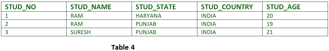
Example 1 – In relation STUDENT given in Table 4,
FD set: {STUD_NO -> STUD_NAME, STUD_NO -> STUD_STATE, STUD_STATE -> STUD_COUNTRY, STUD_NO -> STUD_AGE}
Candidate Key: {STUD_NO}
For this relation in table 4, STUD_NO -> STUD_STATE and STUD_STATE -> STUD_COUNTRY are true. So STUD_COUNTRY is transitively dependent on STUD_NO. It violates the third normal form. To convert it in third normal form, we will decompose the relation STUDENT (STUD_NO, STUD_NAME, STUD_PHONE, STUD_STATE, STUD_COUNTRY_STUD_AGE) as:
STUDENT (STUD_NO, STUD_NAME, STUD_PHONE, STUD_STATE, STUD_AGE)
STATE_COUNTRY (STATE, COUNTRY)
Example 2 – Consider relation R(A, B, C, D, E)
A -> BC,
CD -> E,
B -> D,
E -> A
All possible candidate keys in above relation are {A, E, CD, BC} All attributes are on right sides of all functional dependencies are prime.
4. Boyce-Codd Normal Form (BCNF) –
A relation R is in BCNF if R is in Third Normal Form and for every FD, LHS is super key. A relation is in BCNF iff in every non-trivial functional dependency X –> Y, X is a super key.
Example 1 – Find the highest normal form of a relation R(A,B,C,D,E) with FD set as {BC->D, AC->BE, B->E}
Step 1. As we can see, (AC)+ ={A,C,B,E,D} but none of its subset can determine all attribute of relation, So AC will be candidate key. A or C can’t be derived from any other attribute of the relation, so there will be only 1 candidate key {AC}.
Step 2. Prime attributes are those attributes that are part of candidate key {A, C} in this example and others will be non-prime {B, D, E} in this example.
Step 3. The relation R is in 1st normal form as a relational DBMS does not allow multi-valued or composite attribute.
The relation is in 2nd normal form because BC->D is in 2nd normal form (BC is not a proper subset of candidate key AC) and AC->BE is in 2nd normal form (AC is candidate key) and B->E is in 2nd normal form (B is not a proper subset of candidate key AC).
The relation is not in 3rd normal form because in BC->D (neither BC is a super key nor D is a prime attribute) and in B->E (neither B is a super key nor E is a prime attribute) but to satisfy 3rd normal for, either LHS of an FD should be super key or RHS should be prime attribute.
So the highest normal form of relation will be 2nd Normal form.
Example 2 –For example consider relation R(A, B, C)
A -> BC,
B ->
A and B both are super keys so above relation is in BCNF.
Key Points –
BCNF is free from redundancy.
If a relation is in BCNF, then 3NF is also satisfied.
If all attributes of a relation are prime attributes, then the relation is always in 3NF.
A relation in a Relational Database is always and at least in 1NF form.
Every Binary Relation ( a Relation with only 2 attributes ) is always in BCNF.
If a Relation has only singleton candidate keys( i.e. every candidate key consists of only 1 attribute), then the Relation is always in 2NF( because no Partial functional dependency possible).
Sometimes going for BCNF form may not preserve functional dependency. In that case go for BCNF only if the lost FD(s) is not required, else normalize till 3NF only.
There are many more Normal forms that exist after BCNF, like 4NF and more. But in real world database systems it’s generally not required to go beyond BCNF.
Exercise 1: Find the highest normal form in R (A, B, C, D, E) under following functional dependencies.
ABC --> D
CD --> AE
Important Points for solving above type of question.
1) It is always a good idea to start checking from BCNF, then 3 NF, and so on.
2) If any functional dependency satisfied a normal form then there is no need to check for lower normal form. For example, ABC –> D is in BCNF (Note that ABC is a superkey), so no need to check this dependency for lower normal forms.
Candidate keys in the given relation are {ABC, BCD}
BCNF: ABC -> D is in BCNF. Let us check CD -> AE, CD is not a super key so this dependency is not in BCNF. So, R is not in BCNF.
3NF: ABC -> D we don’t need to check for this dependency as it already satisfied BCNF. Let us consider CD -> AE. Since E is not a prime attribute, so the relation is not in 3NF.
2NF: In 2NF, we need to check for partial dependency. CD is a proper subset of a candidate key and it determines E, which is non-prime attribute. So, given relation is also not in 2 NF. So, the highest normal form is 1 NF.

Comments
Post a Comment